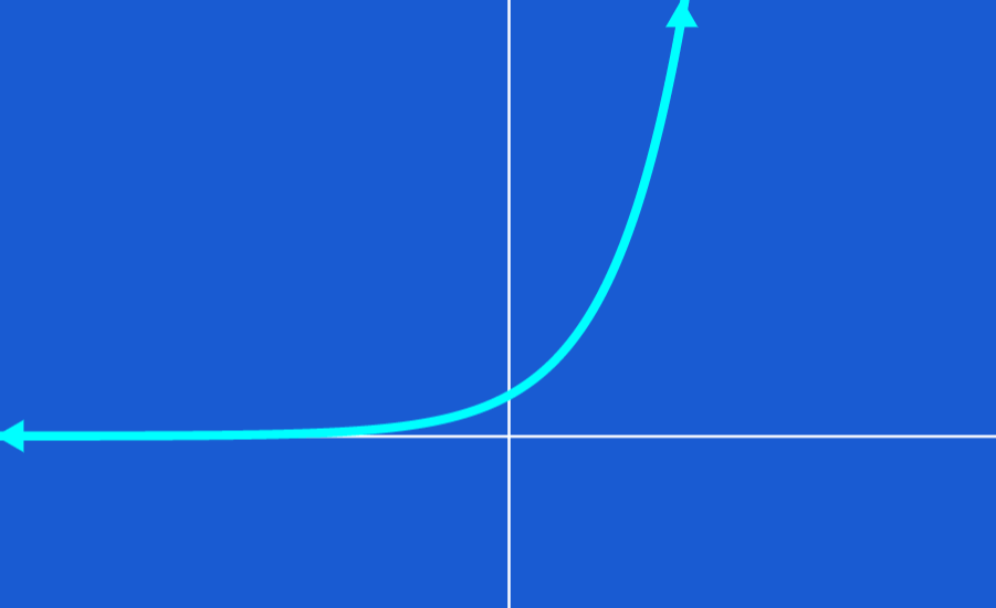
Exponential functions have the form $latex y={{b}^x}$, where $latex b> 0$. Exponential functions are functions that remain proportional to their original value as it increases or decreases. If b>1, the function increases and if 1>b>0, the function decreases.
In this article, we will learn about the graphs of exponential functions and learn about their properties. We will also look at some practice examples.
Definition of exponential functions
In its most basic form, an exponential function can be thought of as a function where the variable appears in the exponent. The simplest exponential function is a function of the form $latex y={{b}^x}$, where b is a positive number.
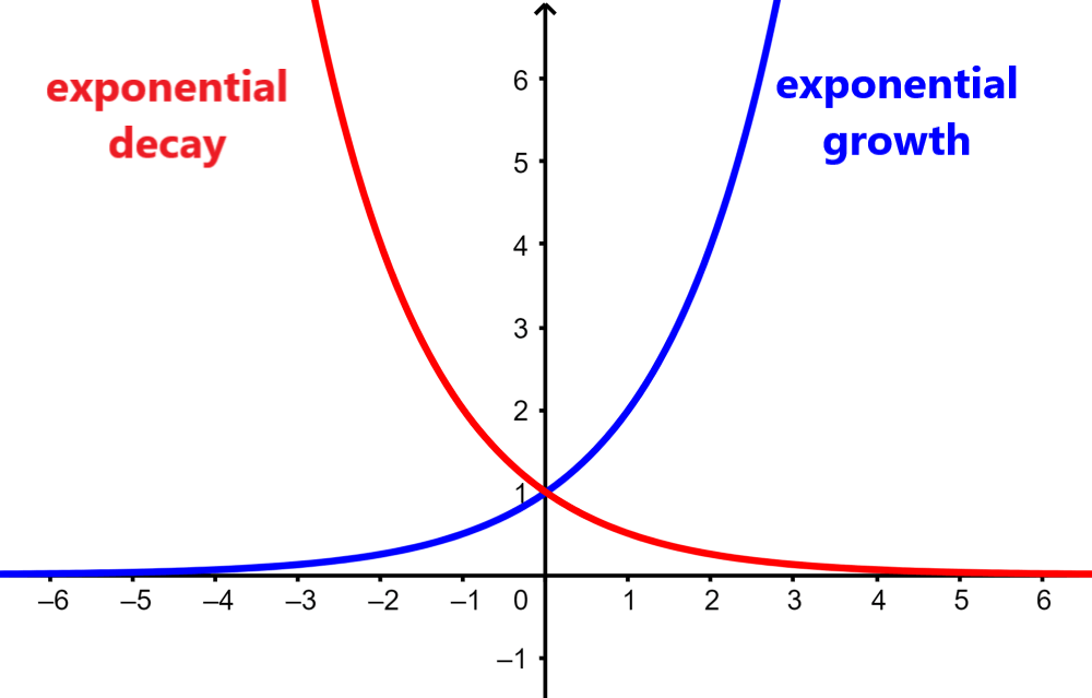
When we have $latex b>1$, the function grows in a way that is proportional to its original value. This is called exponential growth.
When we have $latex 1>b>0$, the function decreases in a way that is proportional to its original value. This is called exponential decay.
Graphs of exponential functions
Let’s look at the following examples of how to graph exponential functions.
EXAMPLE 1
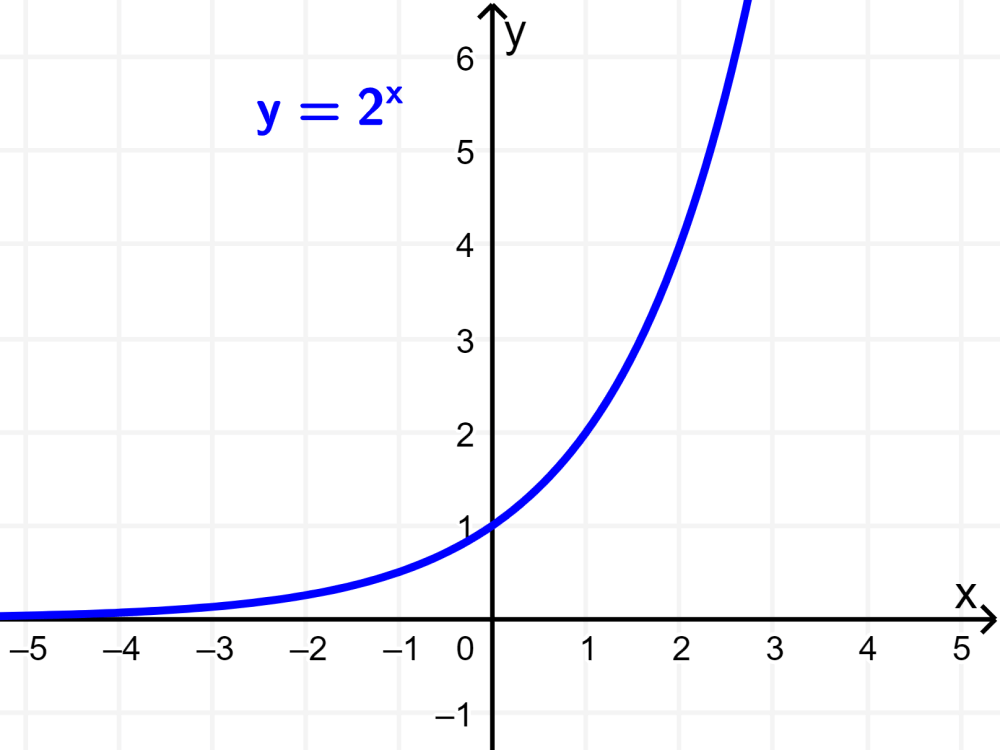
Suppose we want to graph the function $latex y={{2} ^x}$. One way to accomplish this is to choose specific values for x and use them in the function to generate values for y. By doing so, we can obtain the following points:
$latex \left( {-2,\frac{1}{4}} \right),~\left( {-1,\frac{1}{2}} \right),~\left( {0,~1} \right),~\left( {1,~2} \right)$ y $latex ( {2,~4}).$
As we connect these points, we can see that we form a curve that crosses the y-axis through the point (0, 1). The graph grows as the values of x get larger. We can see that this graph tends to infinity as the values of x go to infinity.
Similarly, we can see that as the values of x get smaller and smaller, the curve gets closer and closer to the x-axis. The curve approaches zero as the values of x approach negative infinity. Since the curve never touches the x-axis, we have that the x-axis is a horizontal asymptote of the function.
For any exponential function of the form $latex y={{b}^x}$, where we have $latex b> 1$, we have the point (1, b) on the graph.
EXAMPLE 2
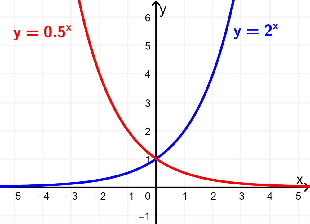
Now, consider the function $latex y={{(\frac{1}{2})}^x}$ when $latex 1> b> 0$. Similar to the previous example, we can graph this exponential function by using several values of x and substituting them in the function to obtain values of y. We can form the following Cartesian coordinates:
$latex \left( {-2, 4} \right),~\left( {-1, 2} \right),~\left( {0,~1} \right),~\left( {1,~\frac{1}{2}} \right)$ y $latex ( {2, \frac{1}{4}}).$
When we connect the points represented by those Cartesian coordinates, we see that the curve that is formed crosses the y-axis through the point (0, 1). The graph of this exponential function decreases as the values of x gets larger.
The graph approaches zero as the values of x tend to infinity. This means that the graph has a horizontal asymptote on the x-axis. We can also observe that the graph tends to infinity as the values of x tend to negative infinity.
For any exponential function of the form $latex y={{b}^x}$, where we have $latex 1>b>0$, we have the point (1, b) on the graph.
By comparing their graphs, we can see that the graph of $latex y=(\frac{1}{2})^x$ is symmetric to the graph of $latex y={{2}^x}$ with respect to the y axis:
Limitation of b to positive numbers
The value of b is limited to numbers greater than 1 due to the following reasons:
• If we have $latex b=1$, the function becomes $latex y={{1}^x}$. We know that 1 raised to any power equals 1, so we would actually have the function $latex y=1$. This function produces a horizontal line, so we would not obtain an exponential function.
• If b is negative, then when we raise b to an even power, we will get positive numbers. However, when we raise b to an odd power, we will get negative numbers. This means that it is impossible to connect the points in a meaningful way, so we will not get a shape similar to the graphs shown above.
Properties of graphs of exponential functions
The following are some of the properties that all exponential graphs share:
• The point (0, 1) is always on the graph of the exponential function of the form $latex y={{b}^x}$, because b is a positive number and all positive numbers raised to the power of zero are equal to 1.
• The point (1, b) is always on the graph of the exponential function of the form $latex y={{b}^x}$. This is because any number b raised to the power of 1 equals b.
• The function $latex y={{b}^x}$ will always produce positive values. Since b is a positive number, we will always get positive values when raised to any power.
• The x-axis is a horizontal asymptote of the function $latex y={{b}^x}$ because the function will always approach the x-axis as x approaches positive or negative infinity, but it never crosses the x-axis since the function is never equal to 0.
See also
Interested in learning more about graphs of functions? Take a look at these pages:

Jefferson Huera Guzman
Jefferson is the lead author and administrator of Neurochispas.com. The interactive Mathematics and Physics content that I have created has helped many students.