The second derivative test is a test that allows us to find the nature of the stationary points of a function. This test tells us that when the second derivative at the point is greater than 0, the point is a minimum. When it is less than 0, the point is a maximum. And when it is equal to 0, the point could be an inflection point.
Here, we’ll learn how to use the Second Derivative Test to find the maximum, minimum, and inflection points of a function.
What is the second derivative test?
The second derivative test is a test that allows us to determine the nature of the stationary points of a function.
The second derivative represents the rate of change of the first derivative. In turn, the first derivative is used to find the slope of the curve at a specific point.
Therefore, the second derivative represents the rate of change of the slope of the function. We can represent this using the following diagram:
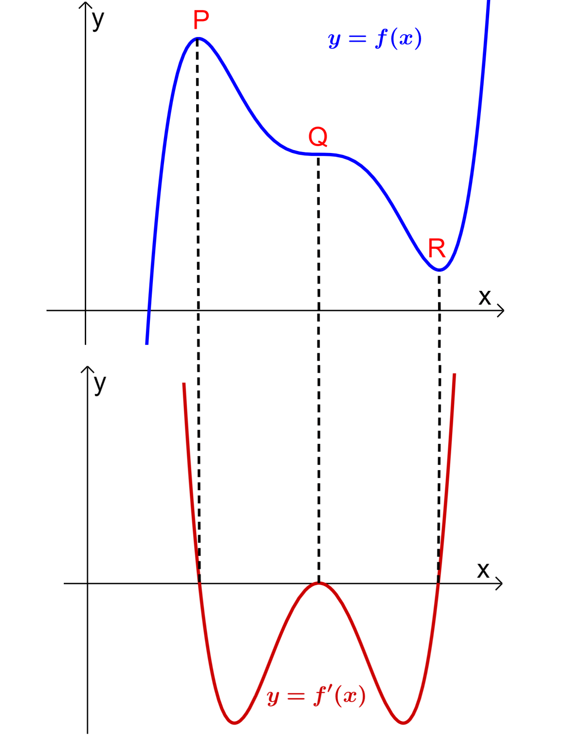
At the top, we have the function $latex y=f(x)$, which has a maximum point (P), a minimum point (R), and an inflection point (Q). At the bottom, we have the graph of the derivative of the function.
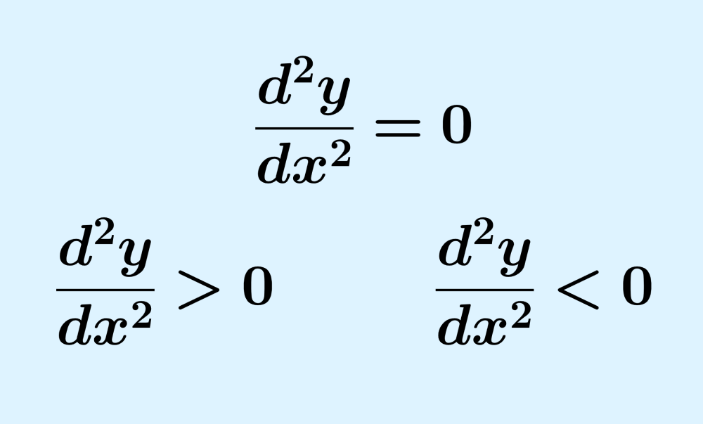
- At the maximum point P, the slope of the derivative of the function (the second derivative) is negative. Then, we have
$latex \frac{d^2y}{dx^2}<0$ at a maximum
- At the inflection point Q, the slope of the derivative of the function (the second derivative) is zero. Then, we have
$latex \frac{d^2y}{dx^2}=0$
Note: There are cases where the second derivative could be zero at a minimum or at a maximum. For this reason, we can examine the sign of the first derivative on each side of the point.
- At the minimum point R, the slope of the derivative of the function (the second derivative) is positive. Then, we have
$latex \frac{d^2y}{dx^2}>0$ at a minimum
In short, the second derivative test tells us that the second derivative of the function is negative at a maximum point, positive at a minimum point, and zero at an inflection point.
How to apply the second derivative test to find stationary points
To find the coordinates of the stationary points of a function, we have to use the first derivative to find these points. We then use the second derivative to determine its nature.
Therefore, we find the stationary points by following these steps:
Step 1: Find the derivative of the function.
Step 2: Find the x-coordinates of the stationary points. For this, we use the derivative from step 1 and form an equation. That is, we have $latex \frac{dy}{dx}=0$.
Step 3: Use the x-coordinates of the stationary points in the original function to find the y-coordinates.
Step 4: The points from step 3 are the stationary points. We use the second derivative to determine the nature of these points.
When $latex \frac{d^2y}{dx^2}<0$, we have a maximum point. When $latex \frac{d^2y}{dx^2}>0$, we have a minimum point. When $latex \frac{d^2y}{dx^2}=0$, we could have an inflection point (confirm with the first derivative).
Second derivative test – Examples with answers
EXAMPLE 1
Find the stationary points of the function $latex f(x)=-x^3+3x+1$ and determine their nature.
Solution
Step 1: Start by finding the derivative of the function:
$latex f(x)=-x^3+3x+1$
$latex f'(x)=-3x^2+3$
Step 2: Forming an equation with the derivative and solving for x, we have:
$latex -3x^2+3=0$
$latex -3x^2=-3$
$latex x=\sqrt{3}$
$latex x_{1}=1~~$ or $latex ~~x_{2}=-1$
Step 3: Use the values of x found to find the y-coordinates:
$latex y_{1}=-(1)^3+3(1)+1$
$latex y_{1}=3$
$latex y_{2}=-(-1)^3+3(-1)+1$
$latex y_{2}=-1$
The stationary points are (1, 3) and (-1, -1).
Step 4: Use the second derivative to determine the nature of the two stationary points found:
$latex f^{\prime \prime}(x)=-6x$
When $latex x=1$, we have $latex f^{\prime \prime}(x)<0$ and when $latex x=-1$, we have $latex f^{\prime \prime}(x)> 0$.
Therefore, the maximum point is (1, 3) and the minimum point is (-1, -1).
EXAMPLE 2
Find the stationary points of $latex f(x)=2x^3-6x$ and determine their nature.
Solution
Step 1: The derivative of the function is:
$latex f(x)=2x^3-6x$
$latex f'(x)=6x^2-6$
Step 2: Form an equation with the derivative to find the x-values of the stationary points:
$latex 6x^2-6=0$
$latex 6x^2=6$
$latex x^2=\sqrt{1}$
$latex x_{1}=1~~$ or $latex ~~x_{2}=-1$
Step 3: Using the x values in the function, we find the y values:
$latex y_{1}=2(1)^3-6(1)$
$latex y_{1}=-4$
$latex y_{2}=2(-1)^3-6(-1)$
$latex y_{2}=4$
Step 4: Now, we use the second derivative to determine the nature of these points:
$latex f^{\prime \prime}(x)=12x$
When $latex x=1$, we have $latex f^{\prime \prime}(x)>0$ and when $latex x=-1$, we have $latex f^{\prime \prime}(x)< 0$.
The minimum point is (1, -4) and the maximum point is (-1, 4).
EXAMPLE 3
What are the stationary points of the function $latex g(x)=x^3 – 3x^2 + 3x+1$?
Solution
Step 1: The derivative of the given function is:
$latex g(x)=x^3 – 3x^2 + 3x+1$
$latex g'(x)=3x^2-6x+3$
Step 2: Form an equation with the derivative and solve by factoring to find the stationary points:
$latex 3x^2-6x+3=0$
$latex 3(x^2-2x+1) = 0$
$latex 3(x-1)(x-1) = 0$
$latex x=1$
Step 3: The y-coordinates of the stationary points are:
$latex y=(1)^3 – 3(1)^2 + 3(1)+1$
$latex y=2$
Step 4: Now, we can classify the stationary points using the second derivative of the function:
$latex g^{\prime \prime}(x)=6x-6$
When $latex x=1$, we have $latex f^{\prime \prime}(x)=0$. So the point (1, 2) is an inflection point.
EXAMPLE 4
Find the coordinates of the stationary points of the function $latex f(x)=x^3-6x^2-15x+1$.
Solution
Step 1: We can find the derivative of the function as follows:
$latex f(x)=x^3-6x^2-15x+1$
$latex f'(x)=3x^2-12x-15$
Step 2: Find the stationary points by forming an equation with the derivative and solving by factoring:
$latex 3x^2-12x-15=0$
$latex 3(x^2-4-5)=0$
$latex 3(x-5)(x+1)=0$
$latex x_{1}=5~~$ or $latex ~~x_{2}=-1$
Step 3: The y-coordinates of the points are:
$latex y_{1}=(5)^3-6(5)^2-15(5)+1$
$latex y_{1}=-99$
$latex y_{2}=(-1)^3-6(-1)^2-15(-1)+1$
$latex y_{2}=9$
Step 4: Using the second derivative, determine the nature of the points found:
$latex f^{\prime \prime}(x)=6x-12$
When $latex x=5$, we have $latex f^{\prime \prime}(x)>0$ and when $latex x=-1$, we have $latex f^{\prime \prime}(x)< 0$.
Therefore, the point (5, -99) is a minimum point and (-1, 9) is a maximum point.
EXAMPLE 5
What are the stationary points of $latex f(x)=x^4+4x^3+1$?
Solution
Step 1: Finding the derivative of the function, we have:
$latex f(x)=x^4+4x^3+1$
$latex f'(x)=4x^3+12x^2$
Step 2: Forming an equation with the derivative and solving for x, we find the stationary points:
$latex 4x^3+12x^2=0$
$latex 4x^2(x+3)=0$
$latex x_{1}=0~~$ or $latex ~~x_{2}=-3$
Step 3: The y-coordinates of the stationary points are:
$latex y_{1}=(0)^4+4(0)^3+1$
$latex y_{1}=1$
$latex y_{2}=(-3)^4+4(-3)^3+1$
$latex y_{2}=-26$
Step 4: We use the second derivative to determine the nature of the stationary points:
$latex f^{\prime \prime}(x)=12x^2+24x$
When $latex x=0$, we have $latex f^{\prime \prime}(x)=0$ and when $latex x=-3$, we have $latex f^{\prime \prime}(x)> 0$.
The point $latex x=0$ could be a turning point. By using the values $latex x=0.1$ and $latex x=-0.1$ in the first derivative, we get slopes with the same sign, so the point is indeed an inflection point.
The inflection point coordinates are (0, 1) and the minimum point coordinates are (-3, -26).
Second derivative test – Practice problems

What is the minimum point of the function $latex f(x)=-2x^4+10x^2-8$
Write the coordinates in the input box.
See also
Interested in learning more about derivatives and stationary points? You can look at these pages:

Jefferson Huera Guzman
Jefferson is the lead author and administrator of Neurochispas.com. The interactive Mathematics and Physics content that I have created has helped many students.