Kinematic Equations for Constant Acceleration

The Five Fundamental Kinematic Equations for Constant Acceleration

The kinematic equations are a set of equations that allows us to calculate the different quantities involved when an object is moving with a constant acceleration. The quantities we are concerned with are

• $latex s=$ displacement
• $latex u=$ initial velocity
• $latex v=$ final velocity
• $latex a=$ acceleration
• $latex t=$ time

Here are the five equations of motion:

Here are the equations along with an explanation of their components:

1. $latex v = u + at$: This equation expresses that the change in velocity is equal to acceleration times the time interval.
2. $latex s=\frac{u+v}{2}\times t$: This equation presents displacement as the product of the average velocity (the sum of the initial and final velocities divided by 2) and the time.
3. $latex s=ut+\frac{1}{2}at^2$: This means that an object’s displacement is the product of the initial velocity and time plus one-half of the acceleration times the square of the time.
4. $latex s=vt-\frac{1}{2}at^2$: This is a rearranged version of the third equation, which is helpful when initial velocity is not given or considered.
5. $latex v^2=u^2+2as$: This conveys that the square of the final velocity is equal to the square of the initial velocity plus twice the acceleration times the displacement.

Note: Each equation is used under specific circumstances and contains particular information about the object’s motion. Knowing which equation to use in different scenarios is crucial in accurately solving kinematic problems.

---

Choosing the Correct Kinematic Equation

Choosing the appropriate kinematic equation relies heavily on the variables outlined within each individual problem. Therefore, start by writing down the quantities which we know, and the quantity we want to find.

Referencing the following table can guide you in determining the right equation to use.

Problem	Equation	Starting from rest
Velocity is requested and $latex a$, $latex t$ are given	$latex v=u+at$	$latex v=at$
Displacement is requested and $latex u$, $latex v$, $latex t$ are given	$latex s=\dfrac{u+v}{2}\times t$	–
Displacement is requested and $latex u,~ a$, $latex t$ are given	$latex s=ut+\frac{1}{2}at^2$	$latex s=\frac{1}{2}at^2$
Displacement is requested and $latex v,~a$, $latex t$ are given	$latex s=vt-\frac{1}{2}at^2$	$latex s=vt-\frac{1}{2}at^2$
Time is not given and not requested	$latex v^2=u^2+2as$	$latex v=\sqrt{2as}$
Velocity is constant ($latex a=0$)	$latex v=\dfrac{s}{t}~$ or $latex ~s=vt$	–

Note: This table shows the simplified forms of these equations applicable when dealing with objects starting from rest, initial velocity equal to 0 or $latex u=0$.

Process for solving problems with the kinematic equations

Most problems related to the kinematic equations can be solved using the following procedure:

Step 1: Create a list with the quantities we know and the quantities we want to find.

Step 2: Choose the equation which links these quantities. The table above can serve as a guide.

Step 3: Substitute in the known values and solve for the unknown values.

---

Proofs of the Kinematic Equations

The kinematic equations are derived from the definitions of velocity and acceleration.

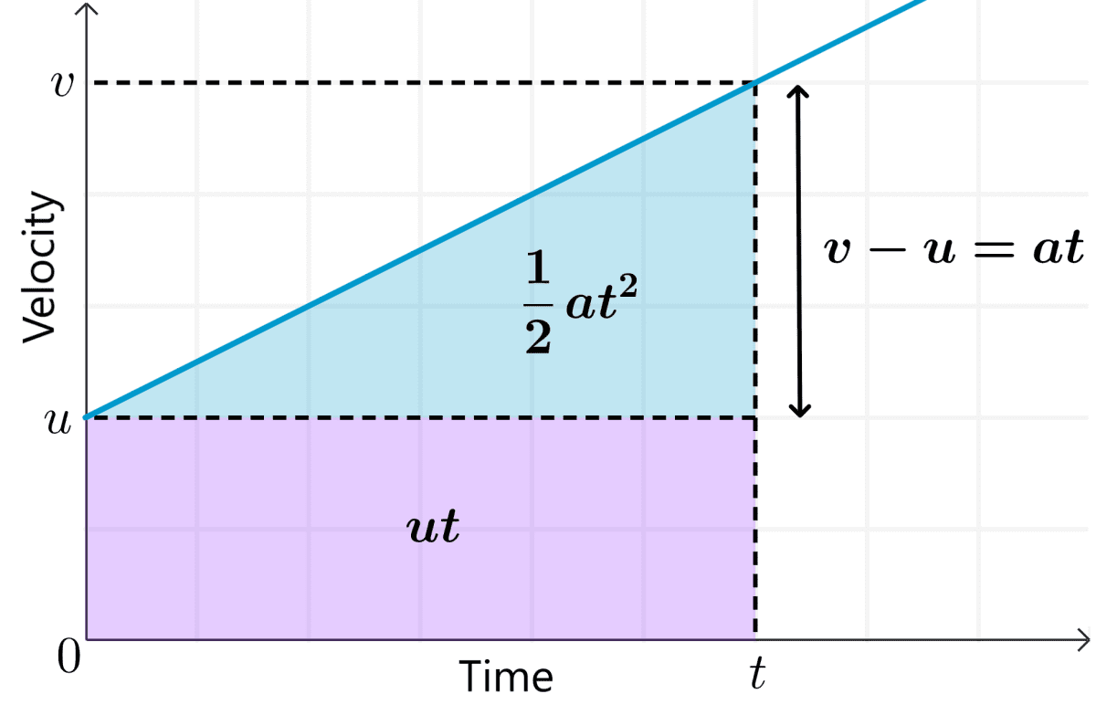
We can use the following velocity vs time graph to help us find the equations. The graph represents the motion of an object with initial velocity $latex u$. After time $latex t$, its final velocity is $latex v$.

Equation 1

The graph shown above displays a straight line, which means that the acceleration $latex a$ is constant. The slope of the line of a velocity vs time graph is equal to the acceleration.

The acceleration or slope of the line is defined as:

$$ a=\frac{v-u}{t}$$

Solving for $latex v$ gives us the first equation of motion:

$latex v=u+at$

Equation 2

In a velocity vs time graph, the area under the graph represents the displacement. Then, the object’s displacement is the shaded area in the following figure:

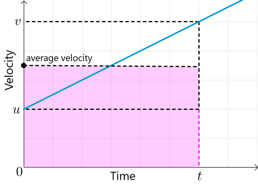
Given that the initial and final velocities are different, we calculated the displacement using the average velocity, which is given by:

$$\frac{u+v}{2}$$

As the shaded area of the figure above is a rectangle, we just multiply the average velocity by the time taken:

$$s=\frac{(u+v)}{2}\times t$$

Equation 3

We can derive equation 3 using equations 1 and 2.

$latex \text{(1)}~~v=u+at$

$latex \text{(2)}~~s=\dfrac{(u+v)}{2}\times t$

Substituting $latex v$ from equation 1 into equation 2, we get:

$$s=\frac{(u+u+at)}{2}\times t$$

$$s=\frac{(2u+at)}{2}\times t$$

$$s=\frac{2ut}{2}+\frac{at^2}{2}$$

$$s=ut+\frac{at^2}{2}$$

This can also be seen in the figure shown above, where the terms $latex ut$ and $latex at^2$ are the areas under the graph representing the displacement.

Equation 4

Similar to equation 3, we just use the equations 1 and 2.

$latex \text{(1)}~~v=u+at$

$latex \text{(2)}~~s=\dfrac{(u+v)}{2}\times t$

However, here we substitute $latex u=v-at$ from equation 1 into equation 2 to get:

$$s=\frac{(v+v-at)}{2}\times t$$

$$s=\frac{(2v-at)}{2}\times t$$

$$s=\frac{2vt}{2}-\frac{at^2}{2}$$

$$s=vt-\frac{at^2}{2}$$

Equation 5

Again, we use equations 1 and 2:

$latex \text{(1)}~~v=u+at$

$latex \text{(2)}~~s=\dfrac{(u+v)}{2}\times t$

We substitute $latex t=\frac{v-u}{a}$ from equation 1 into equation 2 to get:

$$s=\frac{(u+v)}{2}\times \frac{(v-u)}{a}$$

$$2as=(u+v)(v-u)$$

$$2as=v^2-u^2$$

$$v^2=u^2+2as$$

---

Practical Applications of the Kinematic Equations

Everyday Life Examples

The principles behind the kinematic equations play in our day-to-day lives. For instance, when you’re driving, the distance you cover over time and the speed you reach can be calculated using kinematic equations.

Similarly, if you throw a ball upwards, you can calculate the maximum height it will reach and how long it will take to reach the ground again, assuming constant acceleration due to gravity.

Engineering and Technology Applications

In engineering and technology, kinematic equations are used everywhere. For example, mechanical engineers use these equations for designing vehicles and machinery. In the field of robotics, the equations are used to program robots to move in precise ways.

These equations are even used in computer science, playing a crucial role in video game development, particularly in creating more realistic movements and physics in the virtual world.

Scientific Experiments

Kinematic equations are indispensable in various scientific experiments. Physicists often use these equations in designing and interpreting experiments involving motion. For example, in particle physics, researchers studying the behavior of particles under various forces will often use kinematic equations to understand the particles’ motion.

Space Travel and Rocket Science

Perhaps one of the most fascinating applications of the kinematic equations is in space travel and rocket science. When launching a rocket or satellite, scientists and engineers need to calculate the trajectory and velocity needed to escape Earth’s gravitational pull and reach a particular destination.

When landing a spacecraft, they must calculate the deceleration required to ensure a safe landing. All of these calculations involve the kinematic equations, providing a perfect demonstration of their significance.

From these examples, it is clear that the kinematic equations are not just theoretical concepts, but have real-world applications.

---

See also

Interested in learning more about velocity and acceleration? Take a look at these pages: