We can model real-life situations with exponential functions. One of these situations is population decline. There are “standard” formulas that can be used to easily calculate the population or any other quantity by knowing some facts about the situation.
Here, we will look at what the population decrease means and we will learn about its formulas. In addition, we will see several examples with answers of exponential decay that apply these formulas.
Exponential decay summary and formulas
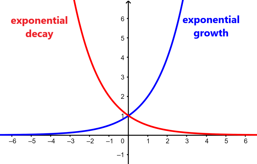
Exponential decay describes the process of reducing an amount by a consistent percentage over a period of time. Exponential decay is very useful for modeling a large number of real-life situations. Most notably, we can use exponential decay to monitor inventory that is used regularly in the same amount, such as food for schools or cafeterias.
The following is the formula used to model exponential decay. It is important to recognize this formula and each of its elements:
| Exponential decay |
| $latex y=a{{(1-r)}^x}$ |
Recall that the exponential function has the basic form $latex y=a{{b}^x}$. Therefore, in the exponential decay formula, we have replaced b with $latex 1-r$. Then, we have:
- $latex a=$ initial amount. Initial amount before decrement.
- $latex r=$ decay factor. Represented as a decimal.
- $latex x=$ time interval.
Many natural events can be modeled using the exponential number e. We can think of e as a universal constant that can be used to represent the growth or decrease that occurs with continuous processes. Furthermore, using e we can also represent exponential growth or decay measured periodically over time.
Therefore, if we have quantities that continuously increase or decrease with a fixed percentage, we can model these scenarios with the following formula:
| Continuous Exponential Decay |
| $latex A=A_{0}{{e}^{kt}}$ |
In this formula, we have:
- $latex A=$ final amount. Amount after decrement.
- $latex A_{0}=$ initial amount. Amount before decrement.
- $latex e=$ exponential. e is approximately equal to 2.718…
- $latex k=$ rate of continuous growth or decline. It is also called the constant of proportionality.
- $latex t=$ time interval.
Exponential decay – Examples with answers
The following examples are solved using what we have learned about exponential decay. Each example has its respective solution, but try to solve the problems yourself before looking at the answer.
EXAMPLE 1
A restaurant served 5,000 customers on Monday. There was a health inspection and the restaurant scored low, so the restaurant served 2,500 customers on Tuesday. On Wednesday, the restaurant served 1,250 customers, and on Thursday only 625 customers.
How many clients will there be after five days starting on Monday?
Solution
We can see that the number of clients decreases by 50% every day. This type of decrement is different from the linear decrease. In linear decrease, the amount that decreases each day would be the same each day.
In this case, the starting quantity is 5000 and the decay factor (r) would be 0.5. x would represent the amount of time in days. Therefore, we can plug these values into the exponential decay formula:
$latex y=a{{(1-r)}^x}$
$latex y=5000{{(1-0.5)}^5}$
$latex y=312.5$
The result is 312.5, but since we cannot have a half client, we round this up to have 313 clients.
EXAMPLE 2
A forest has a population of 1000 birds. Due to deforestation, the bird population is decreasing at a rate of 5% per year. Calculate the size of the bird population after 10 years.
Solution
We have to start by finding the exponential decay function that models the bird population. Then, we use the general form $latex y=a{{(1-r)}^x}$ with the following data:
- $latex a=1000$
- $latex r=0.05$
- $latex t=10$
Therefore, we have:
$latex y=1000{{(1-0.05)}^{10}}$
$latex y=1000{{(0.95)}^{10}}$
$latex y=599$
The bird population after 10 years is 599.
EXAMPLE 3
The cost of a car model decreases in value at a continuous rate of 8% per year. If a car costs 20,000 USD when new, what will it be worth after 5 years?
Solution
This is a case of continuous decay, so we have to use the second formula given above. We use the formula $latex y = a{{e}^{kt}}$ with the following data:
- $latex a=20000$
- $latex k=-0.08$
- $latex t=5$
$latex y=20000({{e}^{-0.08(5)}})$
$latex =20000({{e}^{-0.40}})$
$latex =13406.4$
Therefore, after 5 years the car will cost 13,406.4 USD.
EXAMPLE 4
Rewrite the function from the previous problem in the form $latex y = a {{b}^x}$.
Solution
To write the function $latex y=20000{{e}^{-0.08t}}$ in the form $latex y=a{{b}^x}$, we can use the substitution $latex b={{e}^k}$. Therefore, we have:
$latex b={{e}^k}$
$latex b={{e}^{-0.08}}$
$latex b=0.9231$
⇒ $latex y=20000{{(0.9231)}^x}$
We can also find the value of r using $latex b=1+r$. Therefore, we have:
$latex b=0.9231$
$latex 1+r=0.9231$
$latex r=0.9231-1$
$latex r=-0.0769$
This means that the annual decay rate of the car price is 7.69%.
EXAMPLE 5
Carbon-14 is a radioactive isotope of carbon. Its presence in organic materials is the basis of the radiocarbon dating method. The amounts of carbon-14 present in materials allow for the age of the specimens to be determined.
One artifact had 12 grams of carbon-14. How many grams of carbon-14 will be present in the artifact after 10,000 years if the model $latex A = 12 {{e}^{- 0.000121t}}$ describes the amount of carbon-14 present after t years?
Solution
In this case, we need to find the amount of carbon-14 present after 10,000 years. Therefore, we have to solve for variable A by substituting the value $latex t = 10000$:
$latex A=12{{e}^{-0.000121t}}$
$latex A=12{{e}^{-0.000121(10000)}}$
$latex A=12{{e}^{-1.21}}$
$latex A=3.58$
Therefore, after 10,000 years, the artifact will have roughly 3.58 grams of carbon-14.
EXAMPLE 6
An artifact found at an archaeological site contained 20% of the original carbon-14. Determine the age of the artifact using the exponential decay model for carbon-14 $latex A = A_{0}{{e}^{- 0.000121t}}$.
Solution
In this case, we want to find the age of the artifact, so we have to solve for t.
We do not have specific values of $latex A$ and $latex A_{0}$. However, we know that the carbon-14 found is 20% of the original, so we can use $latex A = 0.2A_{0}$. Therefore, we have:
$latex A=A_{0}{{e}^{-0.000121t}}$
$latex 0.2A_{0}=A_{0}{{e}^{-0.000121t}}$
If we divide both sides by $latex A_{0}$, we have:
$latex 0.2={{e}^{-0.000121t}}$
We take the natural logarithm of both sides to eliminate the exponential:
$latex \ln(0.2)=\ln({{e}^{-0.000121t}})$
$latex \ln(0.2)=-0.000121t$
$latex t=13301$
Therefore, the age of the artifact is approximately 13301 years.
→ Exponential Equations Calculator
Exponential decay – Practice problems
Put into practice what you have learned about exponential decay with the following problems. Solve the problems and select an answer. Check your answer to verify that you selected the correct one.
See also
Interested in learning more about exponential functions? Take a look at these pages:

Jefferson Huera Guzman
Jefferson is the lead author and administrator of Neurochispas.com. The interactive Mathematics and Physics content that I have created has helped many students.